In this vignette, we will retrieve fluorescence intensity values around the position of each spot and display the mean intensity for each spot.
Librairies
To acces the fluorescence intensity values in the Big Data Viewer .h5 file, we need to use the {rhdf5} library.
if (isTRUE(!requireNamespace("cellviz3d"))) {
  stop("Please install {cellviz3d} using:\n",
       " devtools::install_github(\"marionlouveaux/cellviz3d\")")
  # devtools::install_github("marionlouveaux/cellviz3d")
}
#> Loading required namespace: cellviz3d
if (isTRUE(!requireNamespace("rhdf5"))) {
  stop("Please install {rhdf5} using:\n",
       "install.packages(\"BiocManager\"); ",
       "BiocManager::install(\"rhdf5\")")
}
#> Loading required namespace: rhdf5
library(cellviz3d)
library(dplyr)
#>
#> Attaching package: 'dplyr'
#> The following objects are masked from 'package:stats':
#>
#>     filter, lag
#> The following objects are masked from 'package:base':
#>
#>     intersect, setdiff, setequal, union
library(ggplot2)
library(ggridges)
#>
#> Attaching package: 'ggridges'
#> The following object is masked from 'package:ggplot2':
#>
#>     scale_discrete_manual
library(mamut2r)
library(rhdf5)
library(XML)
library(tidyr)
To install {rhdf5}:
# source("http://bioconductor.org/biocLite.R")
# biocLite("rhdf5")
install.packages("BiocManager")
BiocManager::install("rhdf5")
To install {cellviz3d}:
Loading Data
To get the correspondence between spots positions and pixels indices in the .h5 file, we need the .xml file generated by the Big Data Viewer (that was loaded the first time in the Fiji MaMut plugin to start the annotations).
Calculate x, y, z coordinates from registration (setup 0 in Big Data Viewer file)
We now extract information relative to the View registration stored in the BIg Data Viewer file. According to the supplemental information from the Big Data Viewer paper (Pietzsch et al. 2015, Nature methods, Vol.12 No.6), “
read_ViewRegistration() collect all the affine transformations for all timepoints and only setup 0.
prod_affine_registration() concatenate all affine transforms from a given timepoint together.
The lines below apply the affine transform of the corresponding timepoint on each spot coordinates and return a new set of coordinates (POSITION_X_loc, POSITION_Y_loc, POSITION_Z_loc).
Spots_df_loc <- Spots_df %>%
  left_join(Registration_df2, by = c("FRAME" = "Timepoint")) %>%
  rowwise() %>%
  mutate(pos_local = list({#browser();
    res <- crossprod(prod_affine_inv,
              c(POSITION_X, POSITION_Y, POSITION_Z, 1))[1:3,]
      tibble(POSITION_X_loc = res[1],
                 POSITION_Y_loc = res[2],
                 POSITION_Z_loc = res[3])
  })) %>%
  unnest(pos_local, .drop = FALSE)
With the code below you can visually quickly check the positions of the spots before and after applying the affine transforms.
library(rgl)

# Spots location before
plot3d(Spots_df_loc[which(Spots_df_loc$FRAME == 0),
                    c("POSITION_X", "POSITION_Y", "POSITION_Z")],
       size = 20, col = "green")

# Spots location after
plot3d(Spots_df_loc[which(Spots_df_loc$FRAME == 0),
                    c("POSITION_X_loc", "POSITION_Y_loc", "POSITION_Z_loc")],
       size = 20)
Get fluorescence values from MaMuT xml files
Plot distribution of fluorescence per nuclei
We can now display the output of getFluo(). Let’s first select one timepoint only.
The Parhyale dataset has 10 timepoints. The fluorescent data are stored in a list (here called all_cells), of 10 elements (one per timepoints), each of these containing as many elements as the number of spots in the timepoint. In these elements are stored the fluorescence intensities of all the pixels in a cube of 10x10x10 pixels (if using the default cubeSize) around the spot location. Let’s have a look at the distribution of fluorescence of spots at the 6th timepoint, i.e. all_cells[[5]].
singleFrame <- lapply(all_cells[[5]], function(x){
  data.frame(frame = x[[1]], name = x[[2]], fluo = as.vector(x[[3]]))
})

df_singleFrame <- do.call(rbind.data.frame, singleFrame)

head(df_singleFrame)
#>     frame   name fluo
#> 1.1   004 ID1664  203
#> 1.2   004 ID1664  190
#> 1.3   004 ID1664  178
#> 1.4   004 ID1664  178
#> 1.5   004 ID1664  188
#> 1.6   004 ID1664  207

ggplot(df_singleFrame, aes(x = fluo, y = name, fill = name)) +
  geom_density_ridges() +
  theme_ridges() +
  theme(legend.position = "none")
#> Picking joint bandwidth of 44.9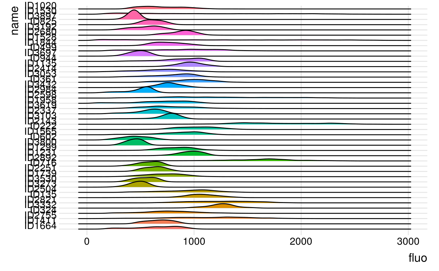
Calculate the mean and median fluorescent value for each spot
mmFluo() calculate the mean and median fluorescent value for each spot.
Spots_df <- mmFluo(Spots_df, all_cells)
#> Joining, by = "name"
#> Warning: Column `name` joining character vector and factor, coercing into
#> character vector
You can visualise the distribution of the mean fluorescent values over the whole movie using {ggplot2}.
ggplot(data=Spots_df, aes(x=meanFluo)) +
  geom_histogram() +
  theme_classic()
#> `stat_bin()` using `bins = 30`. Pick better value with `binwidth`.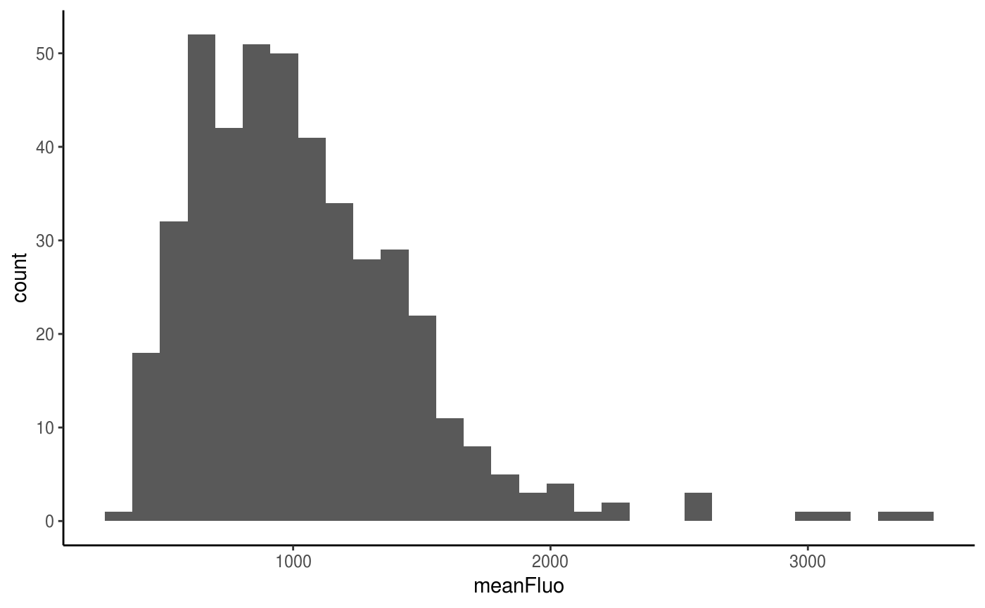
You can also separate the data per timepoint using the facet wrap from {ggplot2} or the geom_density_ridges from {ggridges}:
ggplot(data=Spots_df, aes(x=meanFluo)) +
  geom_histogram() +
  facet_wrap(facets = "frame") +
  theme_classic()
#> `stat_bin()` using `bins = 30`. Pick better value with `binwidth`.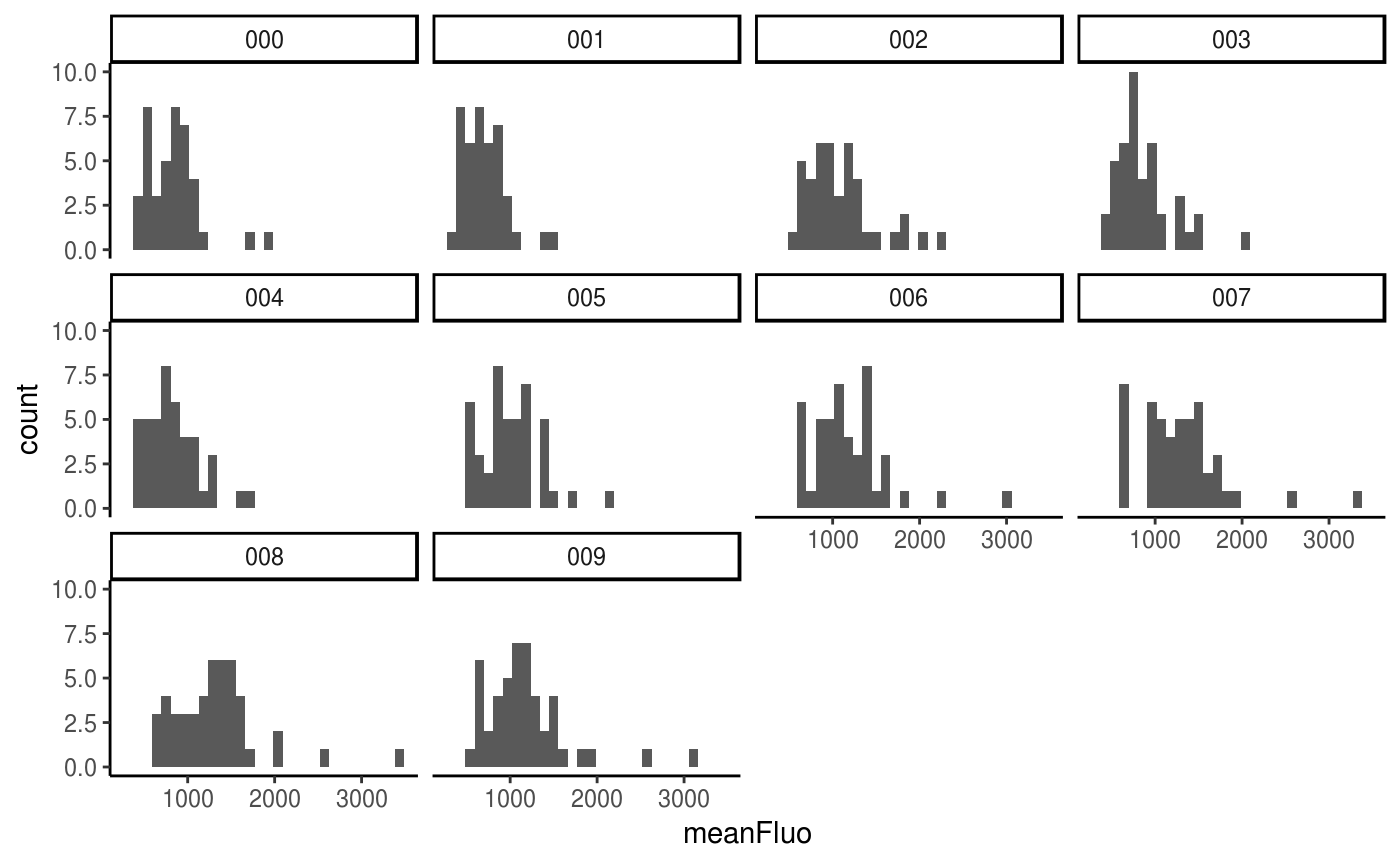
ggplot(Spots_df, aes(x = meanFluo, y = frame, fill = frame)) +
  geom_density_ridges() +
  theme_ridges() +
  theme(legend.position = "none")
#> Picking joint bandwidth of 123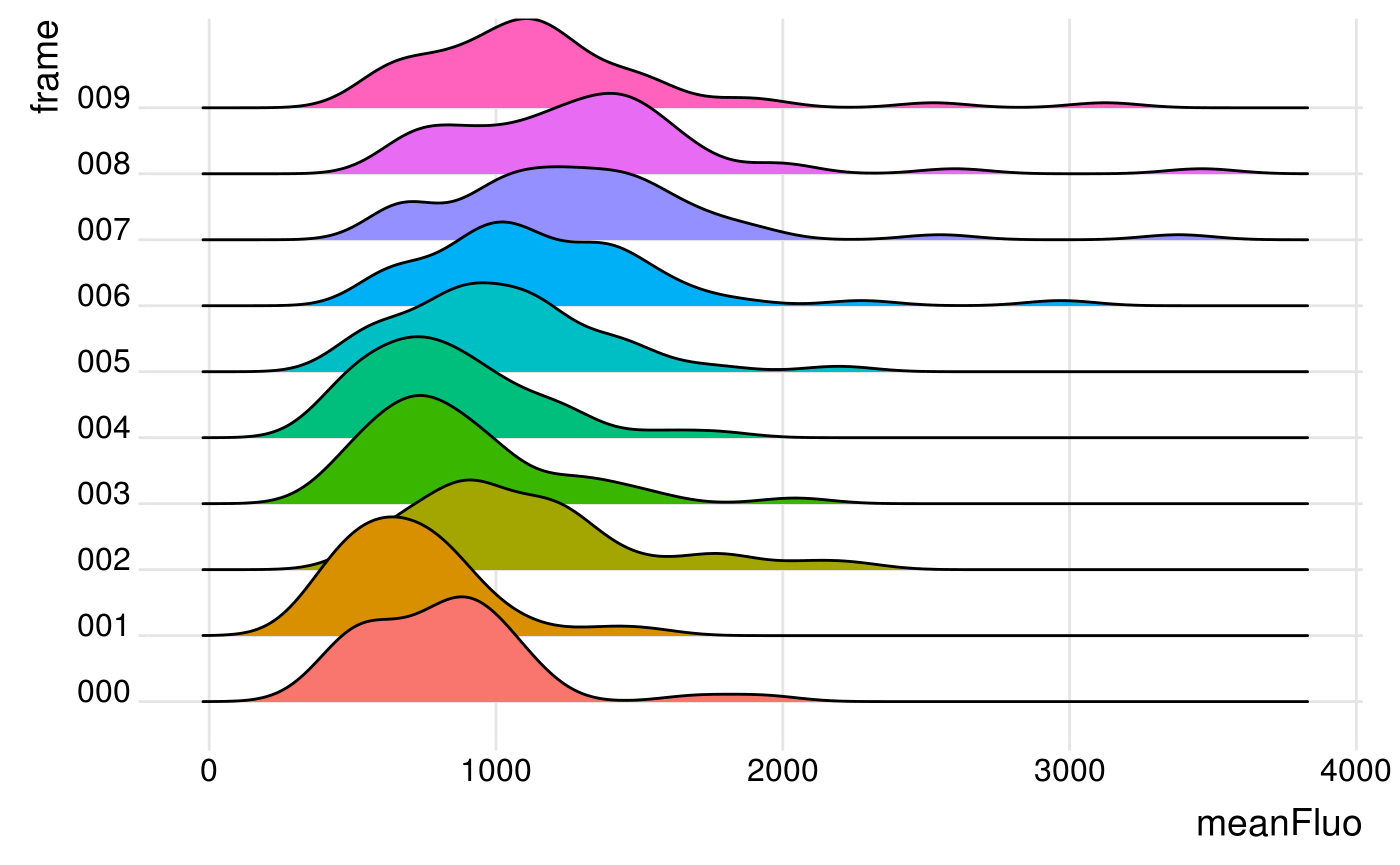
Send back color to MaMuT .xml file
Continuous numerical variables added to Spots_df, like for instance the mean fluorescence intensity value for each spot, can be converted to colors and then converted to integer readable by the MaMuT Fiji plugin and added as a “MANUAL_COLOR” field.
These new “MANUAL_COLOR” field can be added to the MaMuT .xml file. The “MANUAL_COLOR” field is already defined in the features of the MaMuT .xml file. Other new fields are not supported yet by the modifyXML(), as this function does not add new features to define new fields. Below is an example of how to modify the MaMuT .xml file.
Visualise the fluorescence value in 3D
We can visualise the fluorescence intensity values in 3D using the plotlySpots() function from {cellviz3d}, based mainly on the {plotly} library.
Spots_df <- countSpot(Spots_df, FRAME)
#> Joining, by = "FRAME"

plotlySpots(Spots_df = Spots_df,
                x = POSITION_X,
                y = POSITION_Y,
                z = POSITION_Z,
                timepoint = FRAME,
            singleTimepoint = "5",
                number = nb,
                color = meanFluo)
We can also visualise all the timepoints together, using the plotlySpots_all() function from {cellviz3d}, also mainly based on {plotly}.
To go further: normalisation of fluorescence accross the whole movie - different possibilities
- take the fluo of vasculature nuclei as a reference (check first that they do not change too much over time)
# load another mamut file as reference: one or several nuclei in the vasculature tracked over the whole movie.

# MaMuT_ref <- ".xml"
# Spots_df_ref <- Spots.as.dataframe(MaMuT_ref)
# fluo_ref <- getFluo(Spots_df_ref)- normalise to mean/median of all nuclei of the whole movie
- normalise to mean/median of all nuclei of the current frame
- look at variations of the fluorescence intensity by spot over time
#Tn+1 - Tn
diffFluo <- function(Spots_df, all_cells, meancol) {
  meancol <- enquo(meancol)

  Spots_df %>%
    mutate( prev = lag((!!meancol)) ) %>%
    mutate(diffFluo = (!!meancol) - prev)
}

Spots_df <- diffFluo(Spots_df, all_cells, meancol = meanFluo)
To calculate a mean and median fluorescence value per spot + calculate normalised fluorescence accross the whole movie, or for the current frame, all in one go, you can use the mmFluo_all() function.
mmFluo_all(Spots_df, all_cells)
#> Joining, by = c("name", "frame", "meanFluo", "medianFluo")
#> Warning: Column `name` joining character vector and factor, coercing into
#> character vector
#> Joining, by = c("FRAME", "meanFluo_perT", "medianFluo_perT")
#> # A tibble: 441 x 21
#>       ID name  VISIBILITY RADIUS QUALITY SOURCE_ID POSITION_T POSITION_X
#>    <int> <chr> <chr>       <dbl> <chr>   <chr>          <dbl>      <dbl>
#>  1  2115 ID21… 1            14.6 -1.0    0                  0       834.
#>  2  3077 ID30… 1            14.6 -1.0    0                  0       788.
#>  3  1542 ID15… 1            14.6 -1.0    0                  0       865.
#>  4  3398 ID33… 1            14.6 -1.0    0                  0       945.
#>  5  2569 ID25… 1            14.6 -1.0    0                  0       888.
#>  6  1930 ID19… 1            14.6 -1.0    0                  0       836.
#>  7  2956 ID29… 1            14.6 -1.0    0                  0       788.
#>  8  3597 ID35… 1            14.6 -1.0    0                  0      1086.
#>  9   337 ID337 1            14.6 -1.0    0                  0      1046.
#> 10  3025 ID30… 1            14.6 -1.0    0                  0       817.
#> # ... with 431 more rows, and 13 more variables: POSITION_Y <dbl>,
#> #   FRAME <chr>, POSITION_Z <dbl>, frame <fct>, meanFluo <dbl>,
#> #   medianFluo <int>, nb <int>, meanFluo_wholeMovie <dbl>,
#> #   medianFluo_wholeMovie <int>, meanFluo_perT <dbl>,
#> #   medianFluo_perT <dbl>, prev <dbl>, diffFluo <dbl>
Additionnal example: adding a spot in the background to compare fluorescence of background and nuclei
We created an other mamut .xml file named “MaMuT_Parhyale_demo-mamut_withSpotOutside.xml” with one track outside the Parhyale nuclei. The spots in Track ID 42 are located on the background. They have the ID 3964, 3963, 3937, 3965, 3968, 3966, 3962, 3967, and 3961.
fileXML_out <- xmlToList(system.file("extdata", "MaMuT_Parhyale_demo-mamut_withSpotOutside.xml", package = "mamut2r"))We import the spots with Spots.as.dataframe().
We calculate the position of the spots using the registration found above.
Spots_df_loc_out <- Spots_df_out %>%
  left_join(Registration_df2, by = c("FRAME" = "Timepoint")) %>%
  rowwise() %>%
  mutate(pos_local = list({#browser();
    res <- crossprod(prod_affine_inv,
              c(POSITION_X, POSITION_Y, POSITION_Z, 1))[1:3,]
      tibble(POSITION_X_loc = res[1],
                 POSITION_Y_loc = res[2],
                 POSITION_Z_loc = res[3])
  })) %>%
  unnest(pos_local, .drop = FALSE)
We retrieve the fluorescence in a cube of 10x10x10 pixels around each nucleus.
all_cells_out <- getFluo(H5_path = "../data4mamut2r/MaMuT_Parhyale_demo.h5",
                     Spots_df_loc_out,
                     x_px = POSITION_X_loc,
                     y_px = POSITION_Y_loc,
                     z_px = POSITION_Z_loc,
timepoint = FRAME, cubeSize = 5)We calculate the mean and median fluorescence values for all spots.
Spots_df_out <- mmFluo(Spots_df_out, all_cells_out)
#> Joining, by = "name"
#> Warning: Column `name` joining character vector and factor, coercing into
#> character vector
We now display the spots using plotlySpots_all(). When mousing over the spots, we see that the fluorescence values of the spots with the IDs 3964, 3963, 3937, 3965, 3968, 3966, 3962, 3967, and 3961 are very low compared to the fluorescence values of the other spots.